Pseudo-random numbers and sampling from probability distributions
One often needs a source of random numbers for use in stochastic simulations. Since a computer is deterministic, it can’t generate real random numbers, unless one happen to have a quantum random generator at hand, like these. But computers can generate sequences of pseudo-random numbers which are deterministic sequences of numbers which has the same statistical properties as sequences of real random numbers. All of the different random functions in various programming languages, like rand() in C, create sequences of pseudo-random numbers. This post contains my exam notes for the course TDT4270 Statistical image analysis and learning and explains how to generate these sequences, what sampling is and how to sample from any probability distribution.
Pseudo-random number generators
All the different pseudo-random number generators share the property that they in the end will repeat themselves. The length of a unique sequence of pseudo-random numbers, that is the length before the sequence starts repeating itself, is called the generator’s period. For instance the period of the pseudo-random number sequence 1,3,2,4,7,1,3,2,4,7,1,3,2.. is 5. It does not take a genius to see that we want to have a big a period as possible, because the bigger the period, the longer time it takes for the sequence to repeat itself.
The congruential generator
The congruential generator is one of the most common generators. It generates a sequence of pseudo-random numbers X with the simple formula:
\(X_i = (aX_i-1 + c)\mod M
\)
where \(
a,c,X_i \in \lbrace 0,1,..,M-1 \rbrace
\)
M is called the modulus, a the multiplier, c the shift, and \(X_0\) the seed. There are often separate functions for setting the seed. In C its called srand(). The seed is often set to the computers CPU time like this:
srand((unsigned)time(NULL)); |
The reason why we should set the seed is to prevent getting the same sequence when running the same simulations over an over again. If we would get the same sequence for every time we ran the simulation it wouldn’t be very stochastic. Note that in some languages the seed is set automatically.
It is usual to choose M to make the modulus operation easier for the computer to calculate and then to choose a and c to make the period of the generator as long as possible.
Sampling
Sampling in the statistical sense means to retrieve a number. Which number we get is decided by the probability distribution we are trying to sample from. In the previous section, where we were generating pseudo-random numbers we were actually sampling from the uniform distribution. In the uniform distribution every number has equal probability of being the returned sample. If we sample from the standard normal distribution samples around 0 is most likely to be returned.
Sampling from other distributions
So how can we sample from other probability distributions?
Uniform distribution
Recall that in the uniform distribution every number has equal probability of being the returned sample. And as seen in the previous section the congruential generator will return samples from the discrete uniform distribution U(0, M) (0,1,2,…,M-1), where M is the modulus of the generator. If we want to sample from the continuous uniform distribution U(0,1) we can simply divide the sample from the the congruential generator with M. In the C programming language M is defined by the constant RAND_MAX, usually 32767, so sampling from U(0,1) can be done like this:
#include <math.h> #include <time.h> srand((unsigned)time(NULL)); // Set the seed double sample = (double)rand()/RAND_MAX; |
And sampling from a discrete uniform distribution 0,1,2,3,…C-1. Where C is an arbitrary number, can be done like this:
#include <math.h> #include <time.h> srand((unsigned)time(NULL)); // Set the seed int C = 100; // Set to some arbitrary number int sample = rand() % C; // % is the mod operator |
Normal distribution
The other most common distribution is the normal distribution. Several algorithms has been developed for sampling from this famous distribution.
Box-Muller
The most famous of them is probably the Box-Muller algorithm:
First sample U1 and U2 from U(0,1)
\(
\begin{align}
X& = \sqrt{-2\ln U_2}\cdot \cos{2\pi U_1} \\ Y& = \sqrt{-2\ln U_2}\cdot \sin{2\pi U_1}
\end{align}
\)
The returned samples X and Y are two independent samples from the standard normal distribution N(0,1).
To get samples from a normal distributions other then the standard one, you can use this simple formula:
\(
Z = X\cdot\sigma + \mu
\)
Where Z then will be a sample from N(\(\mu, \sigma\)), and X is a sample from N(0,1).
Polar method
The polar method is another method of sampling from the standard normal distribution, which supposedly is faster because it avoids using sine and cosine:
Loop:
Generate \( V_1, V_2\) from the continuous uniform distribution U(-1, 1)
Until: \( W = V_1^2 + V_2^2 < 1[/latex]
[latex]
\begin{align}
C& = \sqrt{-2\frac{\ln W}{W}} \\ X& = C\cdot V_1 \\ X& = C\cdot V_2
\end{align}
[/latex]
The returned samples X and Y are two independent samples from the standard normal distribution N(0,1).
Other distributions
A number of smart direct sampling algorithms for other distributions have been found, and can probably be found on the web by a simple google search.
Making your own sampling algorithms
The direct sampling methods are usually made by using some general sampling methods, and some are made with pure math magic 🙂 Here I explain two of the most common methods of creating algorithms for sampling from a distribution.
Inversion method
If the probability distribution has a cumulative distribution function
[latex]F(x) = P(X \leq x) = \int\limits_{-\infty}^{x} f(t) dt\)
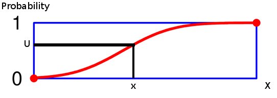
where f(x) is the probability density function, and it has an inverse, we can use the inversion method to create a sampling method. The graph of a cumulative probability function looks something like the figure below:
On the the y axis we have probability from 0 to 1 and along the x axis are all of the values for X.
Since the cumulative distribution function is monotone non-decreasing we can sample a X value from it by retrieving the x value which has the y value equal to some sample u from U(0,1).
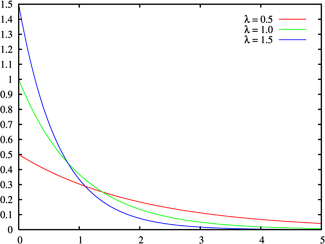
Lets look at an example. Lets say we want to sample from the exponential distribution which has the probability density function:
\(f(x) = \lambda e^{-\lambda x}\)
The cumulative probability function of this PDF is:
\(\int\limits_{0}^{x} f(t) dt = F(x) = 1-e^{-\lambda x}\)
The inverse of F(x) is:
\(
\begin{align}
F(x)& = 1-e^{-\lambda x}\\ e^{-\lambda x}& = 1-F(x)\\ \ln e^{-\lambda x}& = \ln (1-F(x))\\ -\lambda x& = \ln (1-F(x))\\ x& = -\frac{\ln (1-F(x))}{\lambda}\\ F^{-1}(y)& = -\frac{\ln (1-y)}{\lambda}
\end{align}
\)
Since we are just going to input a pseudo-random number u between 0 and 1 in as y we can shorten this as:
\(F^{-1}(u) = -\frac{\ln (u)}{\lambda}\)
So to sample from the exponential distribution we can now use this simple algorithm:
Sample u from U(0,1)
Return sample x where x is:
\(x = F^{-1}(u) = -\frac{\ln (u)}{\lambda}\)
This is a universal method, but it can be slow if there is no fast way to evaluate the cumulative distribution.
Rejection sampling
This method can be used if direct sampling from the probability function f(x) is difficult. If we have another probability distribution g(x) which we know an easy way to sample from and the constraint \(f(x) < M\cdot g(x)[/latex] for M > 1.
The algorithm for rejection sampling is:
Sample x from g(x)
Sample u from U(0,1)
If u < f(x) / Mg(x):
Accept x as a sample from f(x)
else:
Reject x as sample from f(x) and repeat algorithm
Metropolis – A universal sampling algorithm
The metropolis algorithm can generate samples from any probability distribution, but it is slower than direct methods.
The algorithm constructs a Markov chain which has an equilibrium distribution w, which we start by assuming is equal to the distribution we are trying to sample from, w = P(X). So by running the chain long enough we will reach w = P(X). Remember that a Markov chain’s state at time n+1 is dependent only on its state at time n.
The metropolis sampling algorithm
Initialize [latex]X_0\) to some random value
n = 0
Loop until the Markov chain has converged:
Sample y from \(f(X_n,y)\)
Sample u from U(0,1)
\(\text{If } u < min(1, \frac{w_y}{w_{X_n}}) = min(1, \frac{P(y)}{P(X_n)}):[/latex]
[latex]X_{n+1} = y[/latex]
else:
[latex]X_{n+1} = X_n[/latex]
n = n + 1
Return [latex]X_n[/latex] as a sample from P(X)
Where f is a transition function or matrix.
Why does this algorithm work?
If we assume that the variable X is discrete and has d possible states/values. Let S be the set of all possible states:
[latex]S = \lbrace s_1,s_2,..,s_d \rbrace\)
For every step in the Markov chain X moves from its current state \(s_i\) to its next state \(s_j\) with a probability given by the element \(P_{ij}\) in the transition probability matrix P. The distribution of probabilities of all states in S at a time n is given by the distribution \(w^{(n)}\) so that we have:
\(w^{(n)} = (p^n_1, p^n_2, .., p^n_d)\)
and the sum of all these probabilities in the distribution equals to 1.
From the theory of Markov chains there is a theorem that says that if we have a reversible transition probability matrix P so that:
\(w_iP_{ij} = w_jP_{ji}\)
then then chain will converge towards the equilibrium distribution w = P(X).
So have do we insure that we have a transition probability matrix P which is reversible as defined above?
Metropolis answers this by sampling the next state \(s_j\) from row i in symmetric matrix Q and accept the new state with probability:
\(
\alpha_{ij} = min(1, \frac{w_{s_j}}{w_{s_i}}) = min(1, \frac{P(X=s_j)}{P(X=s_i)})
\)
This will create a Markov chain with a transition matrix P where \(P_{ij} = \alpha_{ij}Q_{ij}\)
And here is the proof that this guarantees a reversible Markov chain which insures that the chain will converge to w=P(X):
\(
\begin{split}
P_{ij}& = \alpha_{ij}Q_{ij} \\ w_iP_{ij}& = w_i\alpha_{ij}Q_{ij} \\ &= w_i min(1, \frac{w_j}{w_i})Q_{ij} \\ &= min(w_i, w_j)Q_{ij} \\ &= min(w_i, w_j)Q_{ji} \text{ because Q is symmetric $Q_{ij}=Q_{ji}$} \\ &= w_j min(\frac{w_i}{w_j}, 1)Q_{ji} \\ &= w_j\alpha_{ji}Q_{ji} \\ &= w_jP_{ji}
\end{split}
\)
Hence \(w_iP_{ij} = w_jP_{ji}\)
This was a demonstration of the discrete case, but it holds for the continuous case also were Q then is swapped with a continuous symmetric distribution f instead, for instance the normal distribution with the current state as mean value.


To obtain the cumulative probability function you should integrate from 0 to X in the example, not from -infinite to X.
Very useful, thanks!
You are absolutely right, thanks.
You can also try sampling with the so-called stochastic collocation method- “The Stochastic Collocation Monte Carlo Sampler: Highly Efficient Sampling from ‘Expensive’ Distributions.” Its very easy to implement- even in excel.
I tried the ‘rejection sampling’ approach and it failed. Seems like the success of the algorithm depends upon the value of ‘M’…..
Useful for me.
Will you please send a copy of the electronic version of the book “Stochastic Simulation” ?
Thanks.
Sorry. I don’t have an electronic version of it. I guess you will have to purchase it or read the parts that are online on google: http://www.google.no/books?hl=no&lr=&id=rmGfsJxRDqgC&oi=fnd&pg=PP2&dq=stochastic+simulation+ripley&ots=HYI9tZAtMs&sig=7t97fNZQYS5enXmHSb648hHraC0&redir_esc=y#v=onepage&q=stochastic%20simulation%20ripley&f=false
ok, thanks
Very concise and comprehensive; I like the pieces of information therein.
Many thanks,
Fred S.
Very good explanation! thanks
Helped me a lot! Great collection.
And where can I find the systematic knowledge on sampling from probability distribution? I mean which book?
I will be appreciated a lot if you answer me.
Thanks,
Best.
Yuan Gao.
Nice to hear that someone finds this useful!
You could try the book Stochastic Simulation by Ripley (1987).
http://onlinelibrary.wiley.com/book/10.1002/9780470316726
Thanks a lot.
I will find the book.
The information in your website is really useful, especially for me.
Thanks.
Best,
Yuan Gao