Hopfield network
This neural network proposed by Hopfield in 1982 can be seen as a network with associative memory and can be used for different pattern recognition problems. This post contains my exam notes for the course TDT4270 Statistical image analysis and learning and explains the network properties, activation and learning algorithm of the Hopfield network.
Associative memory
Properties
Learning algorithm
Activation algorithm
Example: Pattern recognition
Associative memory
Lets say you hear a melody of a song and suddenly remember when you where on a concert hearing your favorite band playing just that song. That is associative memory. You get an input, which is a fragment of a memory you have stored in your brain, and get an output of the entire memory you have stored in your brain.
The Hopfield network explained here works in the same way. When the network is presented with an input, i.e. put in a state, the networks nodes will start to update and converge to a state which is a previously stored pattern. The learning algorithm “stores” a given pattern in the network by adjusting the weights. There is off course a limit to how many “memories” you can store correctly in the network, and empirical results show that for every pattern to be stored correctly, the number of patterns has to between 10-20% compared to the number of nodes.
Properties of the Hopfield network
- A recurrent network with all nodes connected to all other nodes
- Nodes have binary outputs (either 0,1 or -1,1)
- Weights between the nodes are symmetric \(W_{ij} = W_{ji}\)
- No connection from a node to itself is allowed
- Nodes are updated asynchronously (i.e. nodes are selected at random)
- The network has no “hidden” nodes or layer
Activation algorithm
A node i is chosen at random for updating. Every node has a fixed threshold \(U_i\) and the nodes output or current state \(s_i\) is set by first calculating the netinput to the node which is the sum of all the input connection multiplied with their weights:
\(
\text{netinput}_i = \sum_{j \neq i} W_{ij}s_j
\)
And then the state is set to 0 or 1 according to this simple rule:
\(
s_i = \left\{ \begin{array}{l l} 0 & \quad \text{ netinput}_i < U_i \\ 1 & \quad \text{ netinput}_i > U_i \end{array} \right.
\)
Learning algorithm
The learning algorithm of the Hopfield network is unsupervised, meaning that there is no “teacher” telling the network what is the correct output for a certain input. The algorithm is based on the principle of Hebbian learning which states that neurons that are active at the same time increase the weight between them, often simplified as “cells that fire together, wire together”.
Suppose we want to learn or “store” a set of patterns P where each pattern p consists of a set of states \(s^p\) in the network we simply loop through all the weights in the network and set them accordingly:
\(
W_{ij} = \sum_{p \in P} (2s_i^p-1)(2s_j^p-1)
\)
By studying the formula above we can see that nodes that have the same state, with a given pattern, will increase the weight between them. While for a pattern where they have opposite states, the weight between them will decrease.
Example: Pattern recognition
How can we use this network to recognize patterns, where the input patterns can be noisy compared to the actual stored patterns?
Lets say we want to recognize which symbol a MxN sized image resembles to a number of stored symbols/images. Also assume that the image is black and white only. One easy way to do this is to have one node for each pixel in the image, so that we have MxN nodes in total. A node is on, i.e. its state is equal to 1, if its pixel is black, and is off, or 0, if its pixel is white.
By first training the network with the symbols/images we want it to learn. And then setting the network in a state given by a input pattern/image which is noisy. The network will after a lot of updates in the nodes state values, according to the activation algorithm, converge to the stored symbol which the input symbol resembles the most.

2 Responses
[…] [2] Erik Smistad, “Hopfield network”, available online at: https://www.eriksmistad.no/hopfield-network/ […]
[…] using recurrent neural network dynamics derived from the Hopfield-Tank-Amari model, the current state of the system (the order of cities the extensions correspond to) influences the […]