Visualizing learned features of a caffe neural network
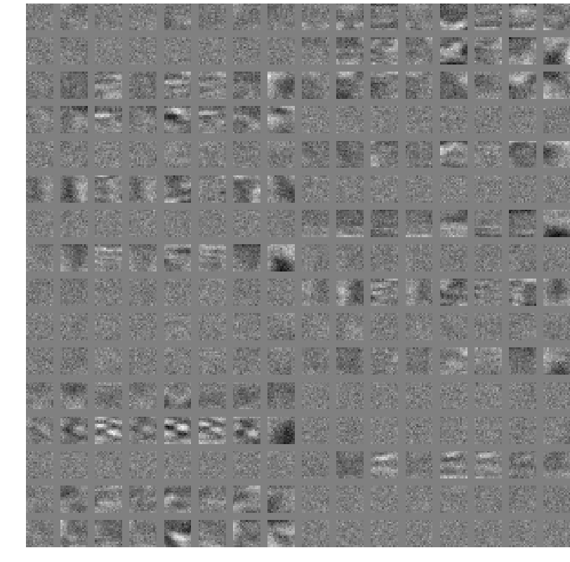
Learned features of a caffe convolutional neural network
After training a convolutional neural network, one often wants to see what the network has learned. The following python function creates and displays an image with all convolutions of a specific layer as shown above. If you supply the function with a filename the image will also be saved on disk.
import numpy as np import matplotlib.pyplot as plt def visualize_weights(net, layer_name, padding=4, filename=''): # The parameters are a list of [weights, biases] data = np.copy(net.params[layer_name][0].data) # N is the total number of convolutions N = data.shape[0]*data.shape[1] # Ensure the resulting image is square filters_per_row = int(np.ceil(np.sqrt(N))) # Assume the filters are square filter_size = data.shape[2] # Size of the result image including padding result_size = filters_per_row*(filter_size + padding) - padding # Initialize result image to all zeros result = np.zeros((result_size, result_size)) # Tile the filters into the result image filter_x = 0 filter_y = 0 for n in range(data.shape[0]): for c in range(data.shape[1]): if filter_x == filters_per_row: filter_y += 1 filter_x = 0 for i in range(filter_size): for j in range(filter_size): result[filter_y*(filter_size + padding) + i, filter_x*(filter_size + padding) + j] = data[n, c, i, j] filter_x += 1 # Normalize image to 0-1 min = result.min() max = result.max() result = (result - min) / (max - min) # Plot figure plt.figure(figsize=(10, 10)) plt.axis('off') plt.imshow(result, cmap='gray', interpolation='nearest') # Save plot if filename is set if filename != '': plt.savefig(filename, bbox_inches='tight', pad_inches=0) plt.show() |
The following is an example of how to use this function
from visualize_caffe import * import sys # Make sure caffe can be found sys.path.append('../caffe/python/') import caffe # Load model net = caffe.Net('/home/smistad/vessel_net/deploy.prototxt', '/home/smistad/vessel_net/snapshot_iter_3800.caffemodel', caffe.TEST) visualize_weights(net, 'conv1', filename='conv1.png') visualize_weights(net, 'conv2', filename='conv2.png') |
As usual the code can be found on my GitHub page

Hi, any hints of how to visualize the filters (Alexnet) in RGB?
Still error comes. I want to view the first 30 activations of the resulting convolutions in every stage. how to write code??????
Thank you for your reply
If I change as such I’m getting the following error
File “/home/tt603lab/.local/install/hed-master/examples/hed/visualize_caffe.py”, line 29, in visualize_weights
result[filter_y*(filter_size + padding) + i, filter_x*(filter_size + padding) + j] = data[n, c, i, j]
IndexError: index 3 is out of bounds for axis 1 with size 3
Kindly plzzzzzzzzzzz help
when trying to visualize last 3 layers of, it gives following error.
line 13, in visualize_weights
filter_size = data.shape[2]
IndexError: tuple index out of range
How can I visualize last layers?
Your last three layers are probably fully connected/dense layers and not convolutional layers. These layers have less dimensions, thus for these types of layers it doesn’t make sense to use the code above.
It is very useful for me. Thanks for this code.
I am using 3D-Unet (3D convolution). I want to visualize the Learned features of this network. The blob of 3D Unet is 5D blobs arranged as (#of samples, #of channels, depth, height, width). I guess we need to change something from your code, could you give me some advice?
Visualising 3D convolutions is not so straightforward as with 2D, you might need to do some 3D volume rendering, or show the 3D convolution weights slice by slice. Or you can apply the convolution one by one on a volume and look at the effects.
how to visualize only the first 30 filters instead of all the filters in a conv1 layer
Change N to 30, and change the range in the two first for loops, for instance to 6 and 5.
When I did your suggestion
Change N to 30, and change the range in the two first for loops, for instance to 6 and 5.
I’m getting the following error
File “/home/tt603lab/.local/install/hed-master/examples/hed/visualize_caffe.py”, line 29, in visualize_weights
result[filter_y*(filter_size + padding) + i, filter_x*(filter_size + padding) + j] = data[n, c, i, j]
IndexError: index 3 is out of bounds for axis 1 with size 3
Ah yes, my bad. It depends if you want filters from all channels or not. You can change the first for loop to: for n in range(N): and the second for loop: for c in range(1): which will only cover filters in the first channel.