3D Gradient Vector Flow Matlab Implementation

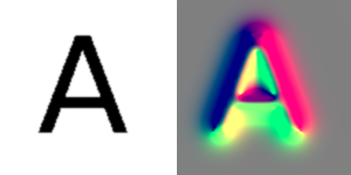
Gradient Vector Flow (to the right) calculated on the volume to the left.
Gradient Vector Flow (GVF) is a feature-preserving diffusion of gradient information. It was originally introduced by Xu and Prince to drive snakes, or active contours, towards edges of interest in image segmentation. But GVF is also used for detection of tubular structures and skeletonization. In this post I present a simple Matlab implementation of GVF for 3D images which I made because I could not find any online. The implementation is a simple extension of Xu and Prince original 2D implementation found at their website.
GVF is the vector field \(\vec V(x,y,z) = [u(x,y,z), v(x,y,z), w(x,y,z)]\) that minimizes the energy function
\( E = \iiint \mu |\nabla \vec V|^2 + |\nabla f|^2 | \vec V-\nabla f|^2 dx dy dz \)where f is the 3D volume itself. This vector field can be found by solving the following Euler equations:
\(\begin{split}\mu \nabla^2 u-(u-f_x)|\nabla f|^2& = 0 \\ \mu \nabla^2 v-(v-f_y)|\nabla f|^2& = 0 \\ \mu \nabla^2 w-(w-f_z)|\nabla f|^2& = 0 \end{split}\)where \( \nabla f = (f_x, f_y, f_z)\). Solving these equations can be done iteratively with the following Matlab function (GitHub Repository of the code can be found here)
1 2 3 4 5 6 7 8 9 10 11 12 13 14 15 16 17 18 19 20 21 22 23 24 25 26 27 28 29 30 31 32 33 34 35 36 37 38 39 40 41 42 43 44 45 46 47 | function [u,v,w] = GVF3D(f, mu, iterations) % This function calculates the gradient vector flow (GVF) % of a 3D image f. % % inputs: % f : The 3D image % mu : The regularization parameter. Adjust it to the amount % of noise in the image. More noise higher mu % iterations: The number of iterations. % sqrt(nr of voxels) is a good choice % % outputs: % u,v,w : The GVF % % Function is written by Erik Smistad, Norwegian University % of Science and Technology (June 2011) based on the original % 2D implementation by Xu and Prince (http://www.iacl.ece.jhu.edu/static/gvf/) % Normalize 3D image to be between 0 and 1 f = (f-min(f(:)))/(max(f(:))-min(f(:))); % Enforce the mirror conditions on the boundary f = EnforceMirrorBoundary(f); % Calculate the gradient of the image f [Fx, Fy, Fz] = gradient(f); magSquared = Fx.*Fx + Fy.*Fy + Fz.*Fz; % Set up the initial vector field u = Fx; v = Fy; w = Fz; for i = 1:iterations fprintf(1, '%d\n', i); % Enforce the mirror conditions on the boundary u = EnforceMirrorBoundary(u); v = EnforceMirrorBoundary(v); w = EnforceMirrorBoundary(w); % Update the vector field u = u + mu*6*del2(u) - (u-Fx).*magSquared; v = v + mu*6*del2(v) - (v-Fy).*magSquared; w = w + mu*6*del2(w) - (w-Fz).*magSquared; end end |
At the boundaries mirror conditions are used and are enforced each iteration by the following function:
1 2 3 4 5 6 7 8 9 10 11 12 13 14 15 16 17 18 19 20 21 22 23 24 | function [f] = EnforceMirrorBoundary(f) % This function enforces the mirror boundary conditions % on the 3D input image f. The values of all voxels at % the boundary is set to the values of the voxels 2 steps % inward [N M O] = size(f); xi = 2:M-1; yi = 2:N-1; zi = 2:O-1; % Coners f([1 N], [1 M], [1 O]) = f([3 N-2], [3 M-2], [3 O-2]); % Edges f([1 N], [1 M], zi) = f([3 N-2], [3 M-2], zi); f(yi, [1 M], [1 O]) = f(yi, [3 M-2], [3 O-2]); f([1 N], xi, [1 O]) = f([3 N-2], xi, [3 O-2]); % Faces f([1 N], xi, zi) = f([3 N-2], xi, zi); f(yi, [1 M], zi) = f(yi, [3 M-2], zi); f(yi, xi, [1 O]) = f(yi, xi, [3 O-2]); end |

If I have a 503050 three-dimensional grid matrix, can I still use this method?
How should the input for the grid graph be entered?
Also, what is the form of the 3D image described in Erik’s provided code?
how can I get the 3D image from streamlines
Hi, I want to detected the aiyway in the CT scans of chest, so I used your GVF3D code to get ‘gvf’ of the scans. But, it seem didn’t work. when I improved the times of iteration, the gradient even disappeared. So what’s the problem. If it is convenient for you, I can send you my code. Thank you in advance.
You probably need several hundred iterations, with matlab this will take a very long time. I have used GPU implementations for this. Still, the gradient should not disappear. Also, use a low value mu, for instance 0.05
Hi Erik,
Can this be applied to anisotropic 3D images as well? For example, if the z dimension of each voxel is 4 times as that of the x and y dimensions.
If so, what are the equations that would be affected?
Yes, it can.
The gradient and Laplacian calculations have to take the voxel spacing into account.
In this code, the gradient and del2 matlab functions are used for this and they do support anisotropic voxel spacing:
http://se.mathworks.com/help/matlab/ref/gradient.html
gradient(F,h1,h2,…) where (h1,h2,…) specifies the spacing for each dimension of F
http://se.mathworks.com/help/matlab/ref/del2.html
L = del2(U,h1,…,hN) specifies the spacing, h1,…,hN, between points in each corresponding dimension of U.
What is the typical values of mu?
Also, how u, v, and w change from one iteration to the another? I have a large 3D volume x*y*z (200*600*180) in which there is a surface (you can see it as a 2D function that maps each (x,y) pair to its z value z = f(x,y)). I want to draw the GVF around the surface f on both sides. Do I really need to set the iteration sqrt(#voxels)? Specifically, I want to know what do I lose if I set the iteration to a lower value to gain speed?
Thanks for the code!
Values I have used for mu with this code are: 0.01-0.05.
You can run GVF until the error falls below a certain threshold instead of setting the number of iterations.
With this GVF solver, the gradient information can move at most one voxel per iteration. Thus, you need at least max(width,height,depth) number of iterations. Having less iterations would reduce the “capture range”. That means that the distance the gradient information has diffused will be shorter. If you are going to use GVF with active contours you in effect have to initialize the contour closer to the surface.
for 2D images does image size is a limitation to gvf deformation?
The image size may affect the number of iterations needed to reach convergence. Thus, in general larger images require more iterations.
the gvf snke is not deforming on images grester than 64X64. It is iterating but not deforming , sforming only a ingle circle. what can be the reason?
Not sure what you mean, but this code is only for 3D images, not 2D.
can you give some examples of snake snake model which use the external force ,gvf?
http://www.mathworks.com/matlabcentral/fileexchange/28149-snake—active-contour
hi, please can you give me an idea about code source matlab_v7 GVF snake because this code don’t run 🙁
can show me your final results image
thank you for your programme
but i don’t understand some steps
why you give the initial u,v and w by Fx ,Fy and Fz respectively and the final result like the filter gaussian
why should enforce the mirror condition on boundary to make boundary gradient 0?
A 0 gradient means that no edge is present, while a gradient unequal to 0 means that there is an edge present. If the gradients were not 0 at the boundaries, GVF would diffuse the gradients from the boundaries of the image. When used with active contours this could draw the contour towards the boundaries, and you don’t want that 😉
i think your way of handle boundary is little different from xu and prince original 2d version. they expand the original data by 1 ring and at the end shrink it.
That is true, but I usually don’t care about the data at the borders and that is why I have omitted that in this implementation.
Thank you very much Erik!
Hello, Canfei, Thank you for your code! But I have a question as follow, when I increase the iteration time, the u,v,w, get bigger and bigger, I don’t know how to handle this problem. when I set iteration time more than 100, for a 3D image, the value of u get more than 1E17.
Try a smaller value for the constant mu, for instance 0.05
This code does not work for 3D data
I’ve used it many times on 3D data, so it should work fine. What type of 3D data are you trying to run it on?
Can you please suggest, how to visualize the output?
Visualizing 3D vector data is not very easy, so I usually just look at one slice at a time. So if you want to look at one z slice (lets say nr 90) of the vector field from GVF, given by u,v and w you can use quiver like this:
figure;quiver(u(:,:,90), v(:,:,90));
What about w? May be we should using:
figure(3);quiver3(Y1(:,:,90),u(:,:,90), v(:,:,90),w(:,:,90));
I am sorry for me to have made a mistake when I ran the program! In fact, the implementation is convergent as you said.Thank you very much!
It is very good for me to find the program! But I have a question as follows: I found that the original 2D implementation is convergent, that is, the outputs are stable. But I found this 3D implementation is not convergent. When I run the paogram in little iterations, the outputs see right. But them see wrong after hundreds of iterations. I think it means that the implementation is not convergent. So I don’t know how to control the iterations by the program. I don’t know if you have faced the same question. Could you give me some help? Thank you very much! Canfei
I found a bug in my code, it is fixed now and should be convergent.